Quickstart

This explains how to quickly and easily plot a catwoman transit using the quadratic limb darkening law. For a more detailed explanation of the parameters, inputs and possible outputs, see the Tutorial tab.

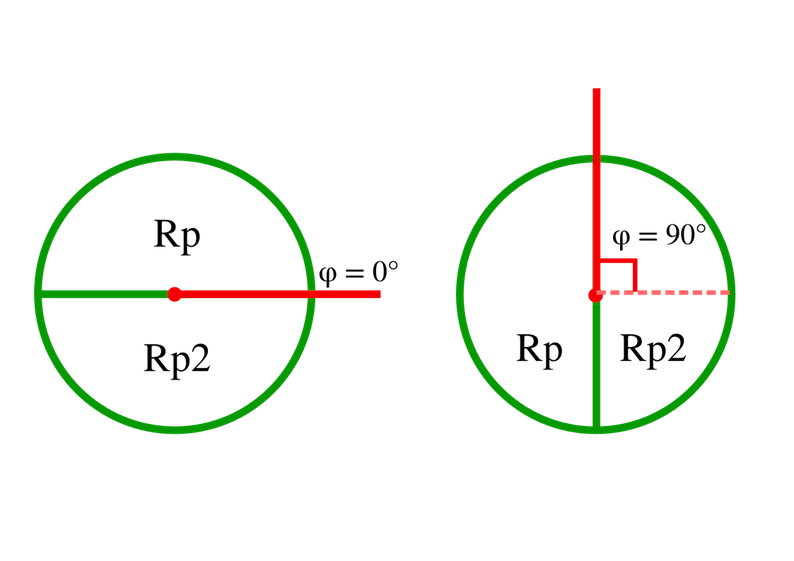
catwoman is a Python package that models asymmetric transit lightcurves where planets are modelled as two semi-circles. The key parameters involved in the asymmetry include params.rp and params.rp2 which define the radius of each semi-circle and params.phi which is the angle of rotation of the top semi-circle defined from -90° to 90° like so:

The first step is to import catwoman and the packages needed for it to run and to plot the results:

import catwoman
import numpy as np
import matplotlib.pyplot as plt

Next, following a similar procedure as to that in batman, initialise a TransitParams object to store the input parameters of the transit:

params  = catwoman.TransitParams()
params.t0 = 0.                          #time of inferior conjuction (in days)
params.per = 1.                         #orbital period (in days)
params.rp = 0.1                         #top semi-circle radius (in units of stellar radii)
params.rp2 = 0.1                        #bottom semi-circle radius (in units of stellar radii)
params.a = 15.                          #semi-major axis (in units of stellar radii)
params.inc = 90.                        #orbital inclination (in degrees)
params.ecc = 0.                         #eccentricity
params.w = 90.                          #longitude of periastron (in degrees)
params.u = [0.1, 0.3]                   #limb darkening coefficients [u1, u2]
params.limb_dark = "quadratic"          #limbs darkening model
params.phi = 0.                         #angle of rotation of top semi-circle (in degrees)

Next make the time array to specify the times we want to calculate the model for:

t = np.linspace(-0.05, 0.05, 1000)

Then, to initialise the model and calculate a light curve:

model = catwoman.TransitModel(params,t)         #initalises model
flux = model.light_curve(params)                #calculates light curve

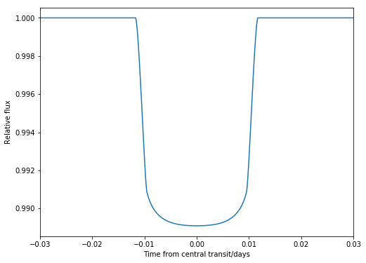
To view the light curve:

plt.plot(t, flux)
plt.xlabel("Time from central transit/days")
plt.ylabel("Relative flux")
plt.show()

To model an asymmetric planet, simply change params.rp and/or params.rp2 and params.phi to change the orientation of the system.

Let’s try this by re-initialising the parameters we want to change so that one of the semi-circles is 0.5% larger than the other and they are orientated with φ = 90°. There is no need to initialise the full model again here, whenever the light_curve function is run, it updates the parameters:

params.rp = 0.1
params.rp2 = 0.1005
params.phi = 90.

Now we calculate the flux again for this new system:

flux2 = model.light_curve(params)

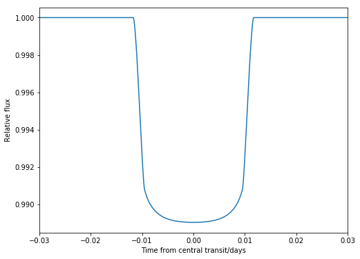
To view this new light curve:

plt.plot(t, flux2)
plt.xlabel("Time from central transit/days")
plt.ylabel("Relative flux")
plt.show()

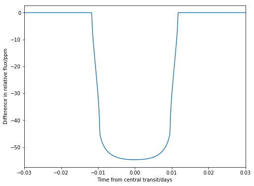
To clearly see the difference between this and the symmetric planet, we can plot the residuals as so:

res = (flux2 - flux)*10**6
plt.plot(t, res)
plt.xlabel("Time from central transit/days")
plt.ylabel("Difference in relative flux/ppm")
plt.show()